Week 6 — Knowing when to stop, and a streaming Pathfinder

Week 5 ended on a promise: the next piece was an online convergence monitor, so a streaming fit could decide when to stop from noisy ELBO estimates rather than a fixed step count. This week I built it — and then carried on into the Phase 2 headline, a Pathfinder that runs on minibatches. Both live in a small lab of their own for now, each with a test suite and a calibration study, so that when I lift them upstream they arrive as clean, self-contained diffs.

Stopping is a change-detection problem, not a plateau

The obvious way to stop a fit is to watch the loss and quit when it stops improving. That does not work here. Each step's loss is a single Monte-Carlo sample of a negative ELBO: its step-to-step noise dwarfs the improvement it is trying to measure, and it is autocorrelated through the parameters. “No new best in the last W steps” just fires on the first unlucky run of noisy samples, long before the fit has actually settled.

The right frame is sequential change detection. Standardize each step's improvement delta_t = loss_{t-1} − loss_t by a robust running scale to get z_t, and accumulate a one-sided CUSUM:

S_t = max(0, S_{t-1} + (kappa − z_t)),   stop when  S_t > h

While the fit keeps improving by more than kappa robust standard deviations per step, S stays pinned at zero; only a sustained run of sub-kappa improvement makes it climb past the threshold h. It is the difference between asking “has it been flat lately?” and asking “has the rate of improvement collapsed and stayed collapsed?”

import pymc as pm
from pymc_streaming_lab import StreamingConvergenceMonitor

with model:
    approx = pm.fit(100_000, callbacks=[StreamingConvergenceMonitor()])
# stops on its own once the ELBO stops improving, and returns the partial fit

The part I did not expect was how easy it is to get the scale wrong. My first cut, tuned only on a clean linearly-decaying curve, called convergence early on 86% of the heavy-tailed traces — it was declaring victory on fits that were still moving. Two changes, both forced by the calibration study rather than guessed, fixed it: estimate the scale from the successive differences of the increments (von Neumann) so a fast-decaying trend can no longer inflate it, and winsorize each standardized increment so a single loss spike contributes only bounded evidence. Together they take the worst-family false-positive rate from that 86% down to 0.6%.

Two-panel operating-characteristic figure. Left: worst-family false-positive rate on a log scale versus median detection delay, for a grid of kappa and h values; points trade delay for fewer false stops, and the default kappa=0.25, h=20 sits at about 70 steps of delay and 0.6% false-positive rate, well below a dashed 5% line. Right: at that default, per-family false-positive bars are 0.6% for linear decay and 0.0% for power-law, heteroscedastic, and heavy-tailed traces, all under the 5% threshold. — Calibrated on 1,000 simulated non-converged ELBO traces per family (linear decay, power-law decay, heteroscedastic and Student-t noise), each over a 20,000-step horizon. The left panel is the cost of the guarantee: buying a lower false-stop rate means waiting a few dozen more steps to be sure. 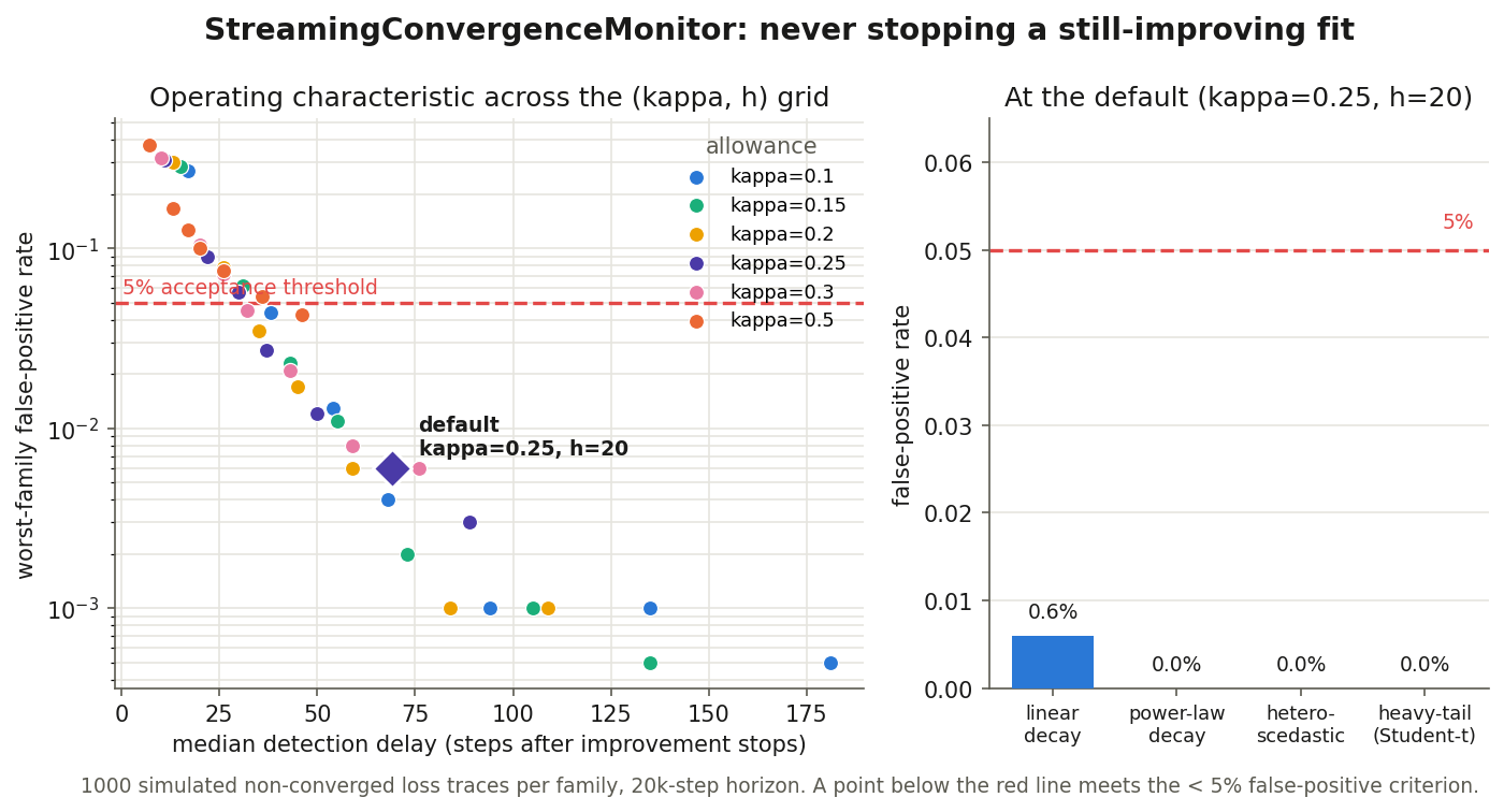The frozen default (`kappa=0.25, h=20`) stops a genuinely-converged fit within ~70 steps while false-stopping a still-improving one at 0.6% — and 0.0% on the three harder families.

Streaming Pathfinder: pair the curvature on one batch

Pathfinder builds a Gaussian posterior approximation from an L-BFGS optimization trajectory, scoring the Gaussian at each iterate by its ELBO and keeping the best one. Upstream, it hands the optimization to SciPy's L-BFGS-B, which assumes a deterministic objective — its Wolfe line search and convergence tests quietly break once the gradients come from minibatches. So the streaming version needs its own quasi-Newton loop. Everything after the optimizer — the diagonal-plus-low-rank Gaussian, the sampler, the Pareto-smoothed importance resampling — is reused from the existing Pathfinder unchanged.

The one subtlety that actually matters is how you form each curvature pair (s, y). The tempting version differences the gradient across two different batches; but then the minibatch noise does not cancel, and s·y goes negative all the time — which L-BFGS cannot use. The fix is to pair on a single batch (Schraudolph et al., 2007): y = ∇f_B(x_new) − ∇f_B(x) with the same B on both sides, so the noise cancels in the difference. Concretely, a fresh batch is written into the model's pm.Data placeholder before each optimization step, so every gradient inside a step is taken on the same batch. Iterate selection is done afterward on one fixed evaluation batch with common random numbers, so the winner is not just whichever step happened to see the luckiest data.

Two checks. On an exactly-Gaussian posterior — linear regression, where Pathfinder should be near-exact — the streaming fit matches the closed-form posterior to Monte-Carlo error:

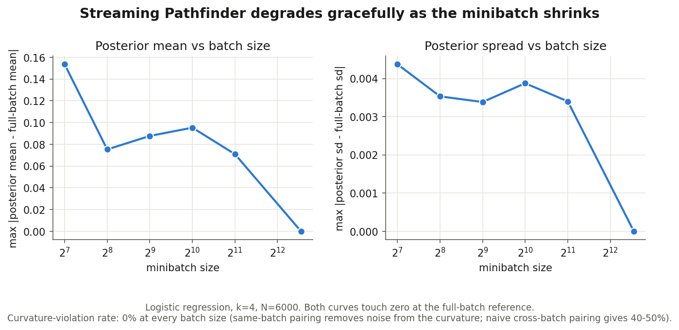
Dumbbell chart of six regression coefficients beta[0] through beta[5]. For each coefficient, the analytic posterior (gray dot with plus-or-minus two standard-deviation bar) and the streaming Pathfinder posterior (blue diamond with matching bar) sit almost exactly on top of each other, with a maximum mean gap of 0.001. — Streaming Pathfinder (blue) against the analytic Gaussian posterior (gray) for a six-coefficient linear regression, full batch. Means agree to within 0.001 and the ±2 sd bars line up; the Pareto-k of the importance-sampling step is 0.27, comfortably in the reliable range.

And as the minibatch shrinks from the full 6,000 rows down to 128, the fit degrades gracefully rather than falling apart — because same-batch pairing keeps the curvature clean, the fraction of rejected curvature pairs stays at 0% the whole way down, where naive cross-batch pairing sits at 40–50%.

Two line charts against minibatch size on a log-2 axis from 128 to full batch. Left: the maximum absolute gap between the streaming posterior mean and the full-batch mean falls from about 0.15 at batch 128 to zero at full batch. Right: the same for the posterior standard deviation, from about 0.004 to zero. Both curves decline smoothly with no blow-up at small batches. — Posterior mean (left) and spread (right) error versus the full-batch reference, as the batch shrinks. The error grows smoothly and modestly as batches get smaller — the expected price of noisier gradients — with no instability, and the curvature-violation rate holds at 0% at every batch size.

Why a separate lab

Neither piece is a one-liner, and both reach into parts of PyMC that the earlier PRs are still moving through review. So rather than pile them onto an open PR, I built each in a small repo of its own — numpy-only where it can be, with its own tests, continuous integration, and the calibration figures above. The point is that each one has a known upstream home and can be lifted there as a self-contained change: the convergence monitor is a Callback subclass for core PyMC, and the streaming Pathfinder slots into pymc-extras right next to the Pathfinder it reuses.

What's next

From here the work goes upstream: the convergence monitor as a callback in core, and the streaming Pathfinder as a dataloader= path alongside the existing fit_pathfinder in extras — the latter aligning with Jesse's new ADVI API, the rewrite I ran into last week. It is also midterm-evaluation week, which is a good moment to have the two remaining proposal pieces working with evidence behind them rather than as plans. More soon.

Links. DataLoader PR #8325 · DataLoader in extras #698 · Trainer PR #8333 · Jesse's new ADVI API #635 · GSoC project page · Mentors @zaxtax · @fonnesbeck