Curvature on a minibatch — a streaming Pathfinder

Week 6 mentioned a streaming Pathfinder in a single line, right next to the convergence monitor. This is the other half of that sentence. Streaming ADVI, the subject of the last few weeks, is the grind-it-out method: thousands of small gradient steps. Pathfinder is the fast one. Getting it to run on data that never lands in memory came down to one subtle fact about how L-BFGS learns curvature, so that is most of what this note is about.

What Pathfinder buys you

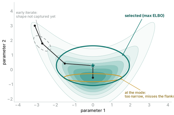
Pathfinder [1] does not optimize a variational family for thousands of steps. It runs a single L-BFGS trajectory from a starting point toward the posterior mode. At each iterate along that path, L-BFGS is already carrying an estimate of the inverse Hessian, and Pathfinder reads a local Gaussian straight off it. It scores each of those Gaussians by ELBO, keeps the best one, and corrects it with Pareto-smoothed importance sampling. Tens of iterations instead of thousands of steps, no learning rate to tune, no step count to guess, and a covariance that carries correlations already, because it is built from curvature rather than a diagonal mean-field assumption.

Contour plot of a banana-shaped posterior with an L-BFGS optimization path descending from the upper left toward the mode at the bottom. Three Gaussian ellipses are drawn along the path: a small dashed gray one at an early iterate labelled shape not captured yet, an amber one at the mode that is wide but very short and misses the upturned flanks, and a large teal one starred as selected max ELBO that covers the bulk of the posterior. — Why Pathfinder keeps the best iterate rather than the last one. Push all the way to the mode and, for anything that is not exactly Gaussian, the local Gaussian there is too tight and misses the flanks. An early iterate has not found the shape yet. The ELBO picks the one in between, which is also what lets Pathfinder stop on its own without a separate convergence check.

Why it does not survive a minibatch

L-BFGS never forms a Hessian. It keeps the last few curvature pairs, s = x' − x and y = ∇f(x') − ∇f(x), and the secant relation y ≈ H·s is what lets those pairs stand in for the curvature. The catch is that y has to be a difference of two gradients of the same function. On a stream, every step sees a different random minibatch. Pair a gradient measured on batch A with one measured on batch B and the difference is dominated by the switch of batch, not by the change in curvature. The pair is noise wearing a curvature costume. The usual health check, s·y > 0, then fails almost half the time, and an inverse-Hessian estimate built from those pairs is meaningless.

Two histograms of the secant test s dot y. On the left, when each gradient of a pair is measured on a different batch, the distribution is very wide and straddles zero, with about 45 percent of the mass below zero shaded as rejected. On the right, when both gradients of a pair are measured on the same batch, the distribution is narrow and entirely positive, with about 0.1 percent rejected. — The same curvature pairs, measured two ways. **Left:** a fresh batch for each gradient. 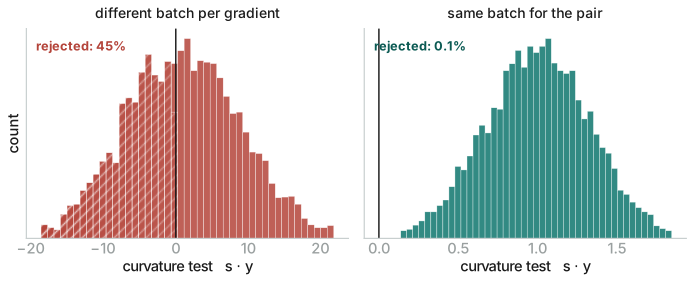The batch swap swamps the signal and about 45% of pairs fail the `s·y > 0` test. **Right:** both gradients of a pair on the same batch. The batch noise cancels in the subtraction and rejections fall to about 0.1%.

The fix is one line of discipline

Measure both gradients of a pair on the same batch [2]. Hold the minibatch fixed for the whole step: compute the gradient, take the L-BFGS step, compute the gradient again on that same batch, and only then form the pair and advance to the next batch. The batch-specific noise is present in both gradients, so it cancels in the subtraction, and what is left is real curvature. In my runs the rejection rate drops from the 45% on the left of the figure to about 0.1% on the right. Holding the batch fixed inside a step has a second benefit: the line search now sees a deterministic objective, so a plain backtracking Armijo search does the job, with none of the Wolfe machinery that a stochastic objective would break.

Being honest about the whole dataset

Choosing which iterate is best only needs a relative comparison, so a fixed evaluation subset is fine there. The final density and its importance weights are a different matter. They have to be the true full-data log density, not a subset scaled up. The scaled subset is unbiased on average, but at any single point it is an estimate with variance, not the density at that point. On one model I measured −797 for the full data against −888 for the scaled subset at the same parameter value, and a gap that size aims PSIS at the wrong target. Computing the full density does not need the data in memory, only a single pass: the prior once, then each batch's likelihood added back at its true weight. That matches model.logp to 1e-6.

One honest wrinkle

While reading my own code I found something that looked wrong. The curvature pairs live in a ring buffer, and once it wraps, the physical column order stops matching the order the pairs were added, while the compact inverse-Hessian form reads those columns by position. That should scramble the covariance. Then I opened the Pathfinder code in pymc-extras and it does exactly the same thing. So this is not something my streaming version introduced. It may be a latent issue upstream instead, and I have written it up with a deterministic reproduction to raise with my mentors rather than quietly working around it. The lesson from last week holds: when something looks alarming, check it against upstream before you panic.

Where it plugs in

None of this is a new inference stack. The streaming Pathfinder feeds on the same DataLoader, the same pm.Data placeholder, and the same total_size scaling that streaming ADVI uses. Only the optimizer changes. Everything after it, the Gaussian sampling and the PSIS correction, is upstream's code reused unchanged. Swapping ADVI for Pathfinder is a different call on the same data contract:

from pymc_streaming_lab import fit_streaming_pathfinder

# same loader, same model, same pm.Data("batch") + total_size=len(loader)
res = fit_streaming_pathfinder(model, loader, num_iters=300, num_draws=2000)
res.samples          # posterior draws, correlations included
res.violation_rate   # fraction of rejected curvature pairs; ~0 with same-batch pairing
res.pareto_k         # PSIS diagnostic; small means the Gaussian was trustworthy

That covers both of PyMC's variational entry points on data that does not fit in memory: the iterative one from the last few weeks, and now the fast one.

References

[1] Zhang, L., Carpenter, B., Gelman, A., & Vehtari, A. (2022). Pathfinder: parallel quasi-Newton variational inference. Journal of Machine Learning Research, 23(306), 1–49.
[2] Schraudolph, N. N., Yu, J., & Günter, S. (2007). A stochastic quasi-Newton method for online convex optimization. AISTATS, 436–443.
[3] Byrd, R. H., Nocedal, J., & Schnabel, R. B. (1994). Representations of quasi-Newton matrices and their use in limited memory methods. Mathematical Programming, 63, 129–156.
[4] Vehtari, A., Simpson, D., Gelman, A., Yao, Y., & Gabry, J. (2024). Pareto smoothed importance sampling. Journal of Machine Learning Research, 25(72), 1–58.

Links. DataLoader in extras #698 · Trainer #710 · GSoC project page · Mentors @zaxtax · @fonnesbeck