Calibrating the stop rule — a CUSUM convergence monitor

Week 6 mentioned an online convergence monitor almost in passing. This week I built it out and calibrated it, and it turned out to be the piece of the streaming-VI work with the most actual statistics in it. So the rest of this note stays on that one component: what problem it solves, why the obvious fixes don't work, and why the thing that does work is a tool from 1954.

The problem: a step count you can't guess

Streaming ADVI needs one number I can't give it: how many optimization steps to run. Stop too early and the approximation hasn't converged; stop too late and, on a dataset that lives on disk, every wasted step is a wasted batch read. In memory you'd just run “plenty” and not care. Out of core, over-running by 10× is real money.

The natural fix is to watch the loss and stop when it flattens. That runs straight into the nature of a streaming ELBO. Each step's loss is a single Monte-Carlo sample of a negative ELBO, evaluated on a random minibatch. Those two sources of randomness make the per-step loss bounce around by far more than the real per-step improvement, routinely 30 to 100 times larger. The signal is buried.

A loss curve over optimization steps. A pale gray jagged line (the measured per-step loss) bounces within a band of about plus/minus 3, while a bold teal line underneath (the true trend) descends smoothly and slowly, flattening out. An annotation points at the trend: the real signal is buried under noise 30 to 100 times larger. — The measured streaming loss (gray) against the true trend it is estimating (teal). 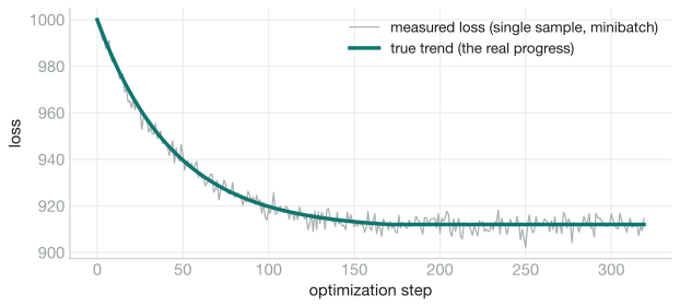A “no new best in the last `W` steps” rule fires on the first unlucky run of upward jumps, long before the fit has actually settled, because it has no way to tell an unlucky patch of noise from a genuine plateau.

The reframe: convergence is a change-detection problem

The trick is to stop asking “has the loss flattened?” and start asking “has the rate of improvement collapsed, and stayed collapsed?” That second question is exactly sequential change-point detection: watch a stream and flag, as fast as possible, the moment its behaviour changes (here, from “still improving” to “only noise left”) while almost never false-alarming before that moment. The classic instrument is the one-sided CUSUM (cumulative sum), introduced by Page in 1954 for exactly this kind of “is the production line still in control?” monitoring [1].

Take the per-step improvement δ_t = loss_t-1 − loss_t, standardize it by a robust noise scale into z_t, and accumulate:

S_t = max(0, S_t-1 + (κ − z_t)), stop when S_t > h

Here is how to read it. κ is an allowance: the smallest improvement rate (in robust standard deviations) still worth waiting for. While the fit improves by more than κ per step, z is large, κ − z is negative, and the max(0,·) pins S at zero. Once improvement collapses, z ≈ 0, S climbs by about κ per step, and it takes roughly h/κ steps of sustained evidence to cross h. A single unlucky step nudges S a little and is immediately pushed back to zero by the next good step.

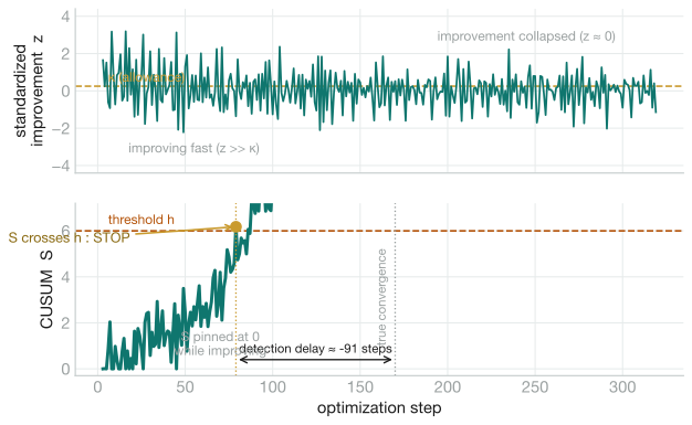
How it works. Top: the standardized improvement z starts far above the allowance κ and collapses to noise after the fit converges. Bottom: the CUSUM statistic S stays pinned at zero while there is real progress, then accumulates the shortfall and crosses the threshold h a controlled number of steps later. It fires on sustained lack of progress, never on a single noisy step.

Why this tool and not, say, a moving-average slope test or a Keras-style patience rule? Because CUSUM is the provably optimal detector for the classic version of this problem, which is what makes it the right starting point. Lorden showed it asymptotically minimizes the worst-case expected detection delay for a given false-alarm rate [2]; Moustakides proved the exact optimality of the CUSUM stopping rule under that criterion [3]. Those proofs assume an i.i.d. change in a known distribution, which a streaming ELBO increment is not, so I don't claim the guarantee transfers verbatim; it is what motivates the choice, and the calibration study below is what earns the defaults. CUSUM also carries O(1) state (one running sum), which is the only kind of memory a streaming monitor can afford, and its two knobs (κ, h) map directly onto the delay-versus-false-alarm trade-off. A windowed slope test has none of these guarantees and drags a lag equal to its window; patience has no controllable false-alarm rate at all.

Making it work on a noisy ELBO

Two details, both forced by the calibration study rather than guessed, are what let the textbook recursion survive a real streaming ELBO.

A trend-robust scale. Standardizing needs the noise scale σ, but early in training the loss falls fast, so measuring the spread of δ directly mistakes the trend for noise and inflates σ. The fix is von Neumann's mean successive difference [4]: estimate σ from |δ_t − δ_t-1|, because differencing annihilates any slowly-varying trend and leaves only noise. For i.i.d. Gaussian increments E|δ_t − δ_t-1| = 2σ/√π, so σ = (√π/2)·E|·|, tracked online with an exponentially-weighted mean. Winsorization. A single-sample MC ELBO has heavy tails, so z is clipped to ±4 before it enters the sum, so one loss spike contributes only bounded evidence.

Calibration, honestly

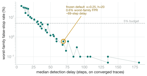
The defaults aren't tuned by eye. I generated 1,000 non-converged loss traces in each of four families (linear and power-law decay, crossed with heteroscedastic and Student-t noise) and measured the operating characteristic: the false-stop rate against the detection delay, over a grid of (κ, h). My first cut, tuned only on a clean linearly-decaying curve, false-stopped 86% of the heavy-tailed traces. The two fixes above took the worst-family false-positive rate to 0.6% at the frozen defaults κ=0.25, h=20, with a median detection delay around 70 steps.

Operating-characteristic scatter: worst-family false-stop rate on a logarithmic y-axis versus median detection delay on the x-axis, for a series of threshold values. The points trace a downward curve: buying a lower false-stop rate costs a longer delay. A dashed line marks a 5 percent budget; all plotted points except the smallest thresholds sit below it. A circled point marks the frozen default kappa 0.25, h 20 at about 0.6 percent false-stop rate and roughly 70 steps of delay. — The cost of the guarantee: a lower false-stop rate buys itself with a few dozen more steps of delay. The frozen default (circled) sits at 0.6% worst-family false stops with a ~70-step delay, comfortably under a 5% budget.

One honest wrinkle

Reviewing my own code, I found the monitor treats a sustained upward move in the loss as evidence to stop: z goes negative, so κ − z grows and S climbs faster. For a fixed objective that's defensible (the fit is diverging, stop it). But in a streaming setting the loss can rise legitimately when the data distribution shifts at an epoch boundary, and there you'd rather keep training and re-converge than declare victory. Whether an upward shift should drain S instead is a design question I'm taking to my mentors; the calibration families are all still-improving, so it doesn't touch the numbers above. I would rather write that down than hide it.

Where it plugs in

None of this reaches into the optimizer. PyMC's pm.fit already exposes a callback protocol (called once per step with the running losses), and the monitor is just an implementation of it that raises StopIteration when S crosses h. The whole thing is numpy-only and O(1) in state, so it lifts into pymc/variational/callbacks.py as a Callback subclass, and it completes the streaming ADVI loop by answering the one question a fixed step count couldn't:

with model:
    approx = pm.fit(100_000, callbacks=[StreamingConvergenceMonitor()])
# a large upper bound for safety; it stops on its own once the ELBO has settled

References

[1] Page, E. S. (1954). Continuous inspection schemes. Biometrika, 41(1/2), 100–115.
[2] Lorden, G. (1971). Procedures for reacting to a change in distribution. Annals of Mathematical Statistics, 42(6), 1897–1908.
[3] Moustakides, G. V. (1986). Optimal stopping times for detecting changes in distributions. Annals of Statistics, 14(4), 1379–1387.
[4] von Neumann, J. (1941). Distribution of the ratio of the mean square successive difference to the variance. Annals of Mathematical Statistics, 12(4), 367–395.
[5] Kucukelbir, A., Tran, D., Ranganath, R., Gelman, A., & Blei, D. M. (2017). Automatic Differentiation Variational Inference. Journal of Machine Learning Research, 18(14), 1–45.

Links. DataLoader in extras #698 · Trainer #710 · GSoC project page · Mentors @zaxtax · @fonnesbeck